Rayleigh-Bénard Convection

One of the simplest setups we can consider is the Rayleigh-Bénard problem, where fluid is contained between two stationary parallel plates which are held at fixed temperatures. If the lower plate is maintained at a higher temperature than the upper plate, then density differences due to temperature can drive convection in the domain. Stronger thermal driving, characterised by a larger Rayleigh number, drives a stronger flow.

In MuRPhFi, we can take advantage of the multiple resolution grid to efficiently simulate this problem at high \(Pr\). Since temp on the coarse grid and sal on the refined grid evolve according to the same equations (up to a different \(Pr\)), we can treat sal as \(-\theta/\Delta\) for the dimensionless temperature of the system. We set activeT=0 to remove the effect of temp on the buoyancy and run the simulation.

2D Visualization

Here, we show the results for \(Ra=10^8\), \(Pr=10\). The simulation was run with a resolution of \(128^3\) on the coarse grid for velocity, and a resolution of \(384^3\) on the refined grid for "temperature". First, we use the script parallel_movie.py to produce a visualisation of a vertical slice of the "temperature" field sal:

Statistics

We can then dive into the statistics output in means.h5 to calculate the dimensionless heat flux due to the convection, the Nusselt number \(Nu\), and the Reynolds number \(Re\). The following are produced from the script plot_time_series.py.

Nusselt number

In Rayleigh-Bénard convection, there are a number of ways to calculate the Nusselt number, all of which should be equivalent (in a time-averaged sense) in a well-resolved, statistically steady state. Firstly, we can measure the conductive heat flux at the top and bottom plates:

\[ {Nu}_\mathrm{pl} = \frac{H}{\Delta} \left.\frac{\partial \theta}{\partial z} \right|_{z=0}, \qquad Nu_\mathrm{pu} = \frac{H}{\Delta} \left.\frac{\partial \theta}{\partial z} \right|_{z=H} \]

The volume average of the heat flux will give us another definition, computed as the sum of conductive and convective contributions:

\[ Nu_\mathrm{vol} = 1 + \frac{\langle w'\theta'\rangle}{\kappa \Delta/H} \]

Substituting this into the equations for kinetic energy \(\langle|\boldsymbol{u}|^2\rangle\) and temperature variance \(\langle\theta^2\rangle\) provide two further definitions, linked to the volume-averaged dissipation rates:

\[ Nu_\varepsilon = 1 + \langle \partial_i u_j \partial_i u_j \rangle / (U_f/H)^2, \qquad Nu_\chi = \langle |\nabla \theta|^2 \rangle / (\Delta/H)^2 . \]

Reynolds number

Since there is no imposed flow and no volume-averaged mean flow in Rayleigh-Bénard convection, we use the volume-averaged kinetic energy \(\mathcal{K}\) to compute a Reynolds number. With this approach, we can also separately compute Reynolds numbers based on the vertical kinetic energy \(\langle w^2\rangle\) and on the horizontal kinetic energy \(\langle u^2 + v^2\rangle\).

As in the Nusselt number plot above, we appear to converge to a statistically steady state for \(t \geq 75 H/U_f\) after the initial transient behaviour.

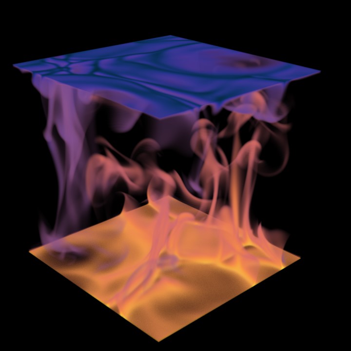
3D Visualization

Finally, we can use the saved 3D snapshots to make a volume rendering of the temperature field. This snapshot highlights the narrow plume structures driving the large-scale circulation at high \(Pr\). The image has been produced using ParaView.